Lineage Definitions in ProVoC

Introduction

This vignette demonstrates some different ways of defining and comparing lineage definitions, including a discussion of why it matters.

Data Prep

This package contains data from Baaijens et al. (2022), as downloaded from NCBI SRA and processed via a custom pipeline (heavily based on GromStole, with some post-processing).

In this paper, they explicitly look for B.1.1.7, B.1.427, B.1.429, and B.1.526. I’m going to add B.1.617.2 to this list, and take this list as given (another vignette will be written to test this assumption).

To make the code run faster, I’ll look at every third day of data.

#library(provoc)
devtools::load_all()

## ℹ Loading provoc

library(lubridate) # ymd()

## 
## Attaching package: 'lubridate'
## 
## The following objects are masked from 'package:base':
## 
##     date, intersect, setdiff, union

library(here) # all paths relative to .git folder

## here() starts at /Users/dbecker/git/DASL/provoc

data(Baaijens)

Baaijens$date <- ymd(Baaijens$date)
dates <- sort(unique(Baaijens$date))
dates3 <- (1:floor(length(dates) / 3)) * 3
dates <- dates[dates3]

b3 <- Baaijens[Baaijens$date %in% dates, 
    c("count", "coverage", "sra", "date", "label")]
b3$mutation <- parse_mutations(b3$label)
head(b3)

##     count coverage         sra       date   label        mutation
## 774  6404    16595 SRR15505103 2021-01-17  ~5700A aa:orf1a:A1812D
## 775 11407    12071 SRR15505103 2021-01-17 ~23401T      aa:S:Q613H
## 776 12519    12661 SRR15505103 2021-01-17 ~23403G      aa:S:D614G
## 777 20293    20794 SRR15505103 2021-01-17 ~14408T  aa:orf1b:P314L
## 778  1885     3207 SRR15505103 2021-01-17 ~16500C aa:orf1b:Q1011H
## 779  4233     4265 SRR15505103 2021-01-17  ~3037T          C3037T

Built-in Constellation Files

The PANGO team used to maintain a GitHub repository called “Constellations” (“Cov-Lineages/Constellations” 2023), which contained mutations that were believed to be more-or-less unique to the lineages. This is no longer updated, but is useful for historical analyses.

This set of lineage definitions is available via the astronomize() function.

astro <- astronomize() |>
    filter_lineages(c("B.1.1.7", "B.1.427", "B.1.429", "B.1.526", "B.1.617.2"))
dim(astro)

## [1]  5 69

astro[, 1:5]

##           aa:S:L452R aa:orf3a:Q57H aa:orf1a:T265I C3037T aa:S:D614G
## B.1.526            0             1              1      1          1
## B.1.1.7            0             0              0      0          0
## B.1.429            1             1              1      1          1
## B.1.617.2          1             0              0      0          0
## B.1.427            1             1              1      1          1

In this matrix, the rows represent the lineages and the columns represent the mutations, with a 1 representing the presence of a mutation in a given lineage.

Notice the use of filter_lineages(). This function gets the rows corresponding to the lineages, but it also ensures that we are only dealing with columns that have at least one “1”. In other words, it only uses mutations that are present in at least one lineage.

I have written a function to visualize this matrix:

plot_lineage_defs(astro)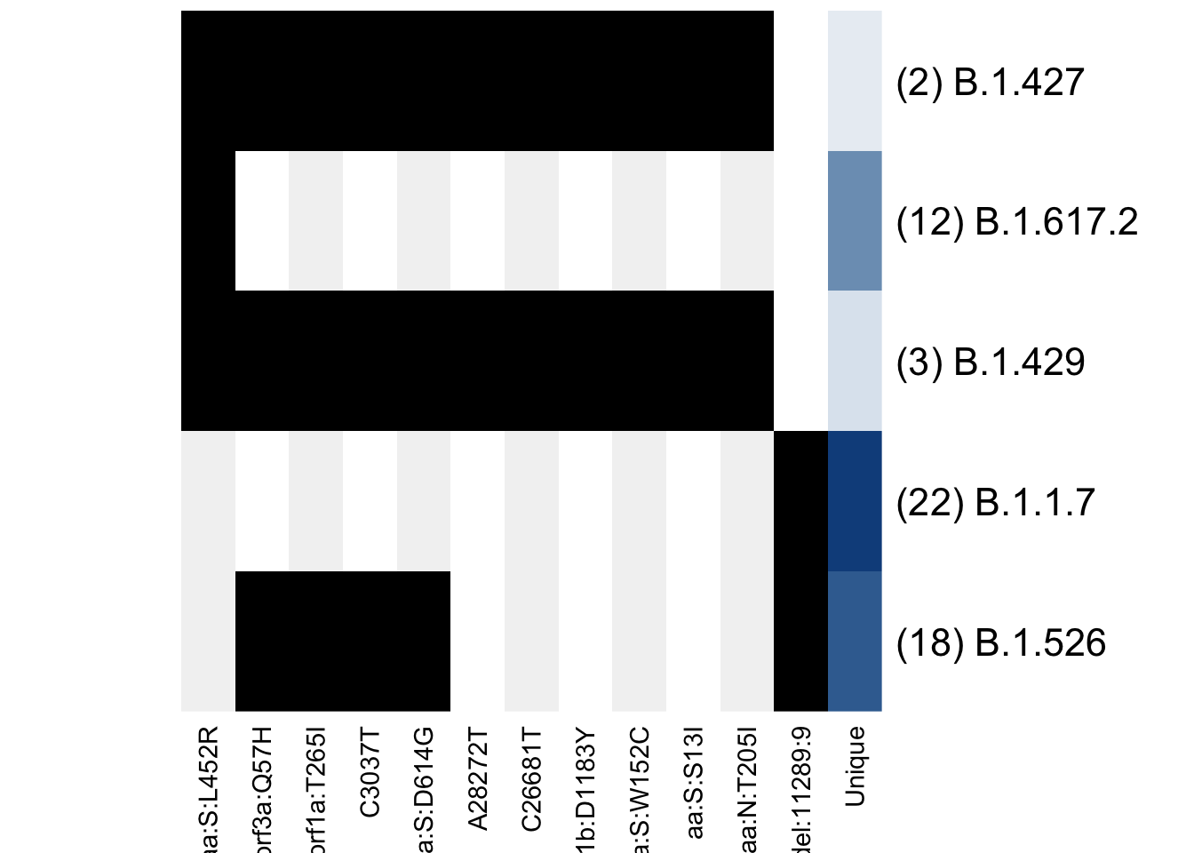

Only the shared mutations are shown, with the last column indicating how many unique mutations remain in each definition. Every other mutation gets a grey background to make it easier to follow a mutation when the matrices are larger.

Usher Barcodes

The Freyja (Karthikeyan et al. 2022; “Andersen-Lab/Freyja” 2024) repository keeps an up-to-date barcodes file, which serves the same purpose as the definitions in constellations.

The usher_barcodes() function will check for this file, then download it if it’s not present in a number of common locations. It’s quite a large file, so I recommend storing the file and using the filter_lineages() function.

bar <- provoc::usher_barcodes(path = "working") |>
    filter_lineages(c("B.1.1.7", "B.1.427", "B.1.429", "B.1.526", "B.1.617.2"))
dim(bar)

## [1]  5 62

Constellations versus Barcodes

Let’s quickly look at the mutations present in astro but not bar, then the mutations present in bar but not astro, as well as mutations that are in both.

plot_lineage_defs2(astro, bar,
    main = "Constellations (red) versus Usher Barcodes (blue)")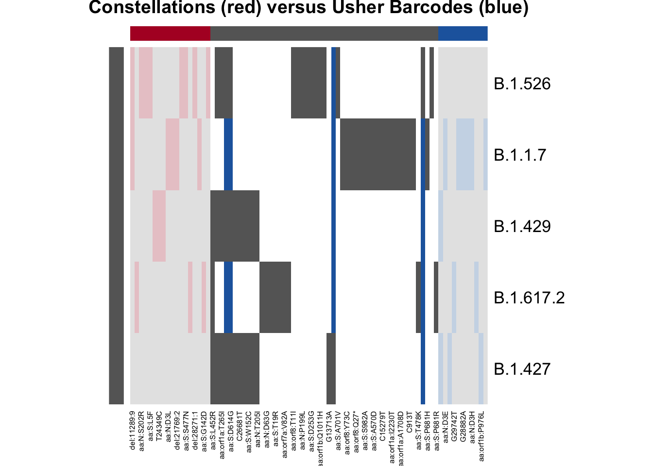

From this plot, we can see that there are quite a few mutations defined in astro but not in bar. The blue bars indicate that the mutation is used in the lineage definition in bar but not astro; there are four mutations defined in both B.1.1.7 and B.1.617.2 by usher barcodes that are not present in the constellations file, and two of those mutations were also present in B.1.429. The barcodes seem to be a little bit more lenient about what mutations to include; constellations tried to get more-or-less “unique” mutations.

Results

Since we chose lineages when choosing the lineage definitions, we can use the convenient “~ .” notation to fit the models with all lineages.

Note that the Baaijens data were processed in such a way that each sample contains the same mutations. This means that each bar you see below is based on the exact same set of mutations. This isn’t necessary, but I believe it improves the interpretability of the results.

library(ggplot2)
library(patchwork) # Patching ggplots together
res_astro <- provoc(count / coverage ~ .,
    lineage_defs = astro,
    data = b3, by = "sra")
res_astro$date <- ymd(res_astro$date)
res_bar <- provoc(count / coverage ~ .,
    lineage_defs = bar,
    data = b3, by = "sra")
res_bar$date <- ymd(res_bar$date)

gg_astro <- autoplot(res_astro, date_col = "date") +
    labs(title = "Constellations")
gg_bar <- autoplot(res_bar, date_col = "date") +
    labs(title = "Usher Barcodes")

gg_astro / gg_bar + plot_layout(guides = "collect") &
    theme_bw() &
    facet_wrap(~ lineage, nrow = 1)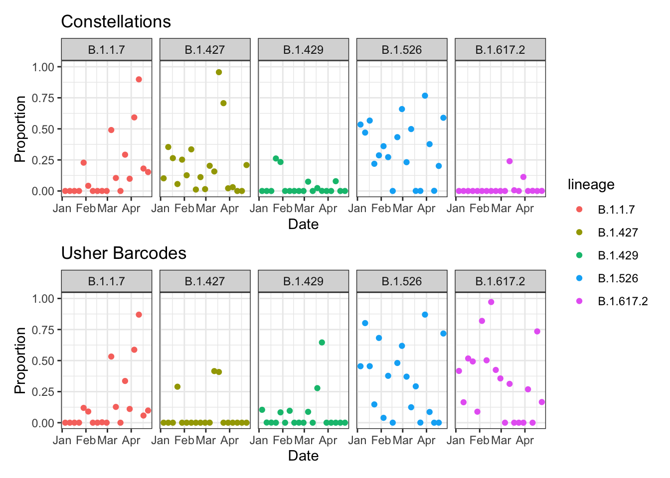

Those are two very different looking plots! We saw before that the lineage definitions are different, but let’s check how they were actually used in the data. The same function can be used from before, which extracts the lineage definitions that were actually used (ignoring any mutations that were part of the definition but not present in the data).

plot_lineage_defs2(res_astro, res_bar,
    main = "Constellations (red) versus Usher Barcodes (blue)")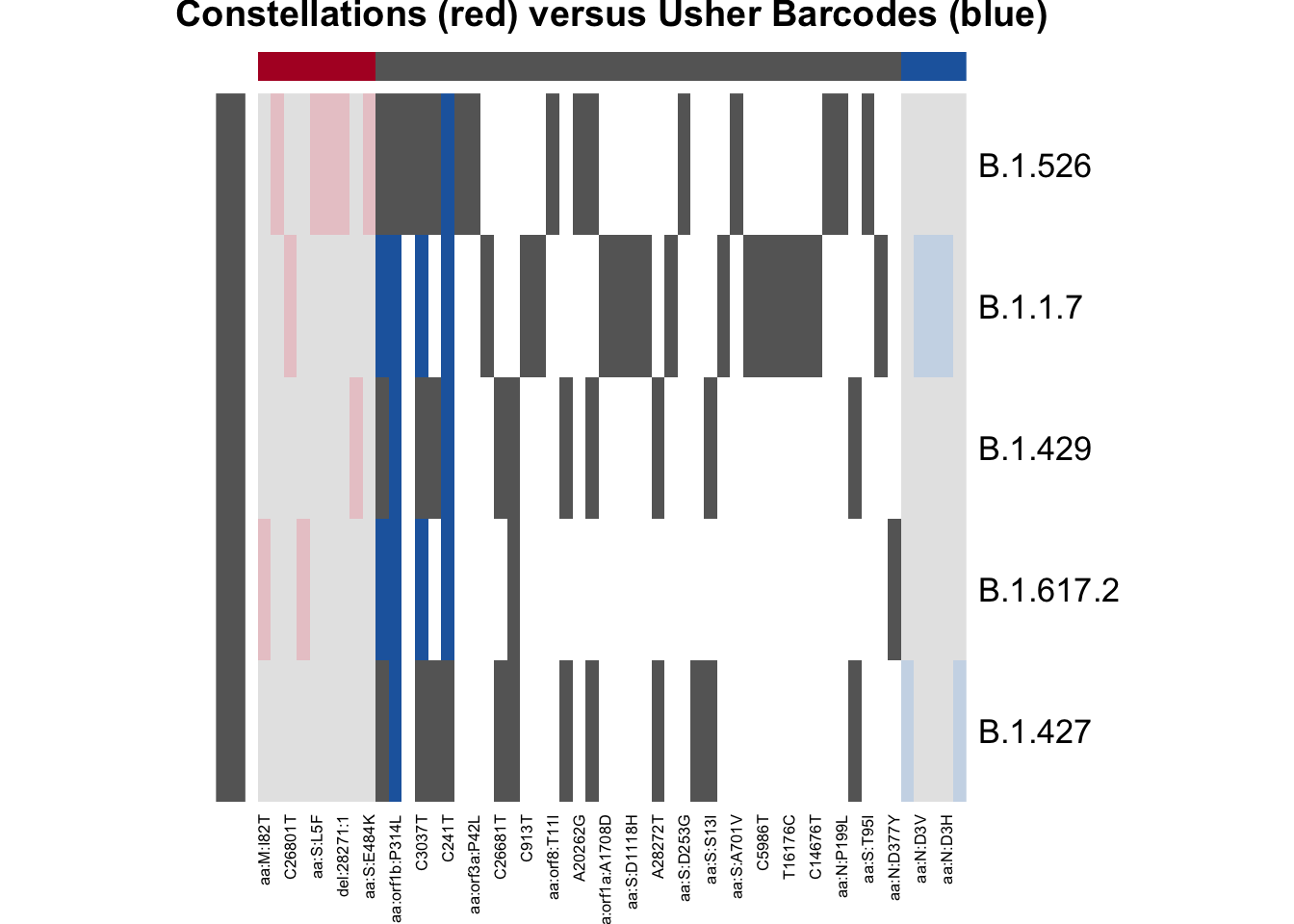

From this result, we can see that constellations only used four mutations to define B.1.617.2! The barcodes used 6! This is because there were only 4 (or 6) mutations in B.1.617.2 that were also present in the data. Let’s dig a little deeper into this.

plot_actual_defs(res_astro, main = "Constellations")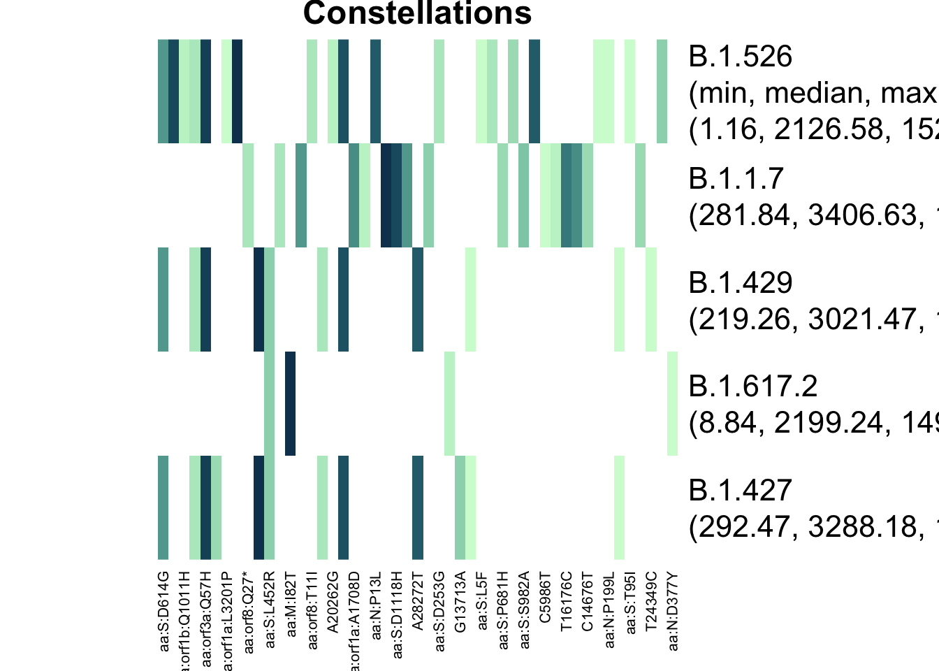

plot_actual_defs(res_bar, main = "Usher Barcodes")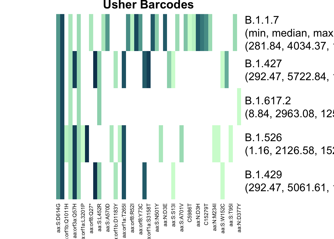

The two different matrices have very different definitions of B.1.617.2, and this explains the difference in results.

Furthermore, B.1.427 and B.1.429 had important differences - the barcodes have more mutations that overlap, meaning that the “de-mixing” algorithm must choose between one or the other. I’ll expand on this in a “Choosing Lineages to Search For” vignette.

LAPIS (CoV-Spectrum)

Since I have not managed to find where to get an API key, the mutations within each lineage were manually downloaded from cov-spectrum.org (Chen et al. 2022). I set the date range to go from 2020-01-01 to 2021-04-27, with the latter being the last sample in the Baaijens data.

The following code is very very hopefully going to change very soon. An API key would be nice, and I desperately need better mutation processing. It is, however, comforting that the column names match with bar, so at least my parsing is consistent!

lineages <- c("B.1.1.7", "B.1.427", "B.1.429", "B.1.526", "B.1.617.2")
lapis_list <- lapply(lineages, function(x) {
    file <- read.csv(here("working", paste0(x, ".csv")))
    file$mutation[file$proportion > 0.8]
})
names(lapis_list) <- lineages
lapis <- lineage_defs_from_list(lapis_list)

# Avoiding parsing deletions, only looking at substitutions
lapis <- lapis[, !grepl("-", colnames(lapis))]
# TODO: user-friendly parsing
colnames(lapis) <- sapply(colnames(lapis), function(x) {
    provoc:::parse_mutation(
        type = "~",
        pos = substr(x, 2, nchar(x) - 1),
        alt = substr(x, nchar(x), nchar(x)))
})

plot_lineage_defs(lapis)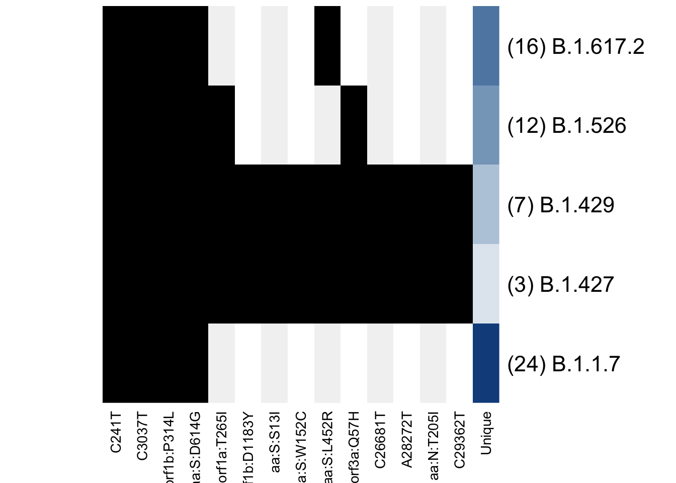

This looks a little different from before. There are 4 mutations that seem to be in every lineage, which doesn’t give the de-mixing algorithm any information about which lineages are present. B.1.1.7 seems to have a lot of unique mutations, which might make the results more accurate (if the mutations truly are unique to B.1.1.7).

Let’s quickly check how this compares to the barcodes:

plot_lineage_defs2(bar, astro)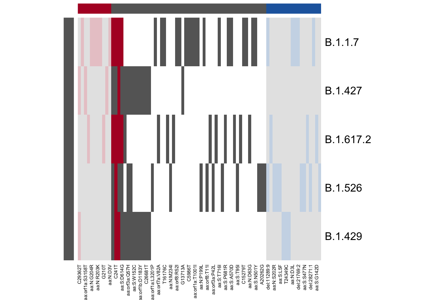

There are a couple mutations in astro but not bar, and a couple in bar but not astro. This is to be expected. However, those red bars in the shared mutation section are noteworthy! They are the same four mutations that we saw in the plot before, which told us that the de-mixing algorithm will have a hard time differentiating the lineages. Let’s check the results.

res_lapis <- provoc(count / coverage ~ .,
    lineage_defs = lapis,
    data = b3, by = "sra")
res_lapis$date <- ymd(res_lapis$date)

gg_lapis <- autoplot(res_lapis, date_col = "date") +
    labs(title = "LAPIS (CoV-Spectrum)")

gg_astro / gg_bar / gg_lapis + plot_layout(guides = "collect") &
    theme_bw() &
    facet_grid(~ lineage)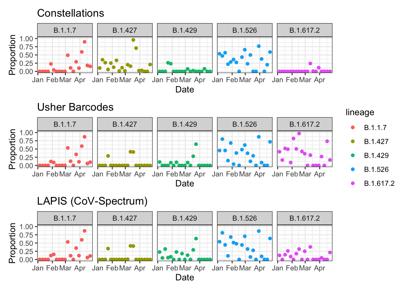

Usher Barcodes and Cov-Spectrum generally agree, but what’s going on with B.1.617.2??? It sort of looks like B.1.429 has taken some of the weight from B.1.617.2, but this is worth looking into. For example, did B.1.429 have mutations that are in B.1.617.2? From the comparison plot, there appear to be a lot of mutations that differentiate B.1.429 and B.1.617.2, so that can’t be it. Maybe it’s the coverage?

plot_actual_defs(res_lapis)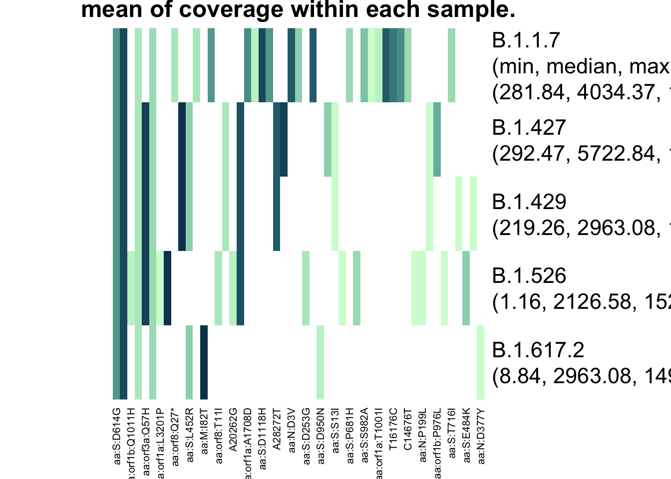

It doesn’t look like the mutations that differentiate B.1.617.2 and B.1.429 had low coverage. The minimum of the average coverages across samples¹ isn’t low for the shared mutations.

I think the primary conclusion here is that the difference in mutations between the barcodes and the lapis definitions is important enough to the demixing algorithm to give the differences in results. Perhaps the next plotting function I make should show something about the frequencies of the mutations in each lineage.

Conclusion

Hopefully this vignette has successfully completed its two goals:

Demonstrate some of the functionality of provoc with lineage definitions.
Demonstrate the importance of choosing good lineage definitions!

References

“Andersen-Lab/Freyja.” 2024. Andersen Laboratory @ Scripps Research.

Baaijens, Jasmijn A., Alessandro Zulli, Isabel M. Ott, Ioanna Nika, Mart J. van der Lugt, Mary E. Petrone, Tara Alpert, et al. 2022. “Lineage Abundance Estimation for SARS-CoV-2 in Wastewater Using Transcriptome Quantification Techniques.” Genome Biology 23 (1): 236. https://doi.org/10.1186/s13059-022-02805-9.

Chen, Chaoran, Sarah Nadeau, Michael Yared, Philippe Voinov, Ning Xie, Cornelius Roemer, and Tanja Stadler. 2022. “CoV-Spectrum: Analysis of Globally Shared SARS-CoV-2 Data to Identify and Characterize New Variants.” Bioinformatics 38 (6): 1735–37. https://doi.org/10.1093/bioinformatics/btab856.

“Cov-Lineages/Constellations.” 2023. CoV-lineages.

Karthikeyan, Smruthi, Joshua I. Levy, Peter De Hoff, Greg Humphrey, Amanda Birmingham, Kristen Jepsen, Sawyer Farmer, et al. 2022. “Wastewater Sequencing Reveals Early Cryptic SARS-CoV-2 Variant Transmission.” Nature, July, 1–4. https://doi.org/10.1038/s41586-022-05049-6.

Devan Becker